Intro and Julia basics
1. Introduction
In this short tutorial, we will introduce the Geophysical Model Generator (GMG). GMG was developed to import and process different kinds of geophysical data. These datasets can then be exported and visualized in Paraview.
The main focus of this tutorial is to learn the basics of the programming language Julia and to show how geophysical datasets can be imported using the tools provided by the Geophysical Model Generator (with the focus on seismic tomographies). At the end, we will also shortly show some basic visualization of selected datasets in Paraview.
The Julia scientific programming language is fast, completely open source and comes with a nice package manager. It works on essentially all systems and has an extremely active user base. Programming in Julia is fairly easy and comparable to programming in MATLAB. If you have experience in MATLAB programming, transitioning to Julia should be relatively smooth.
We are assuming that you are not yet familiar with Julia. The purpose of these exercises is therefore to give you a crash course in how to install it on your system, create a few programs, make plots etc.
2. Installing Julia
The best way to start is to download a recent version of julia (1.6.3) from https://julialang.org (use a binary installer). The recommended debugger for julia is Microsoft Visual Studio Code, where you should install the julia extension. See this page for more info.
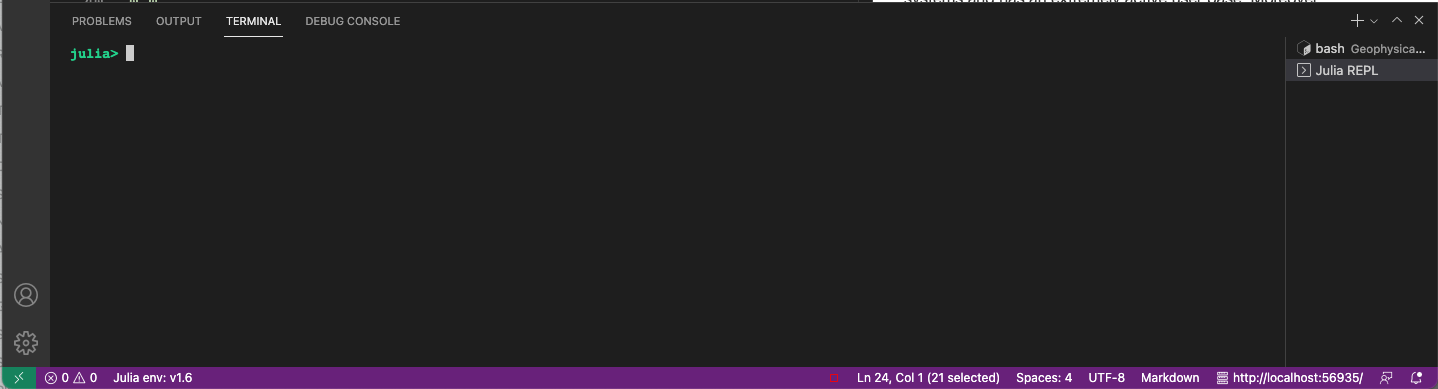
Once this is done (in the order indicated above), you can start the Julia REPL (which stands for read-eval-print-loop, similar to the command window in MATLAB) by typing in the Command Palette (which you find in VS Code under the menu View->Command Palette):
>Julia: Start REPL
This will take a bit of time initially, as it needs to compile. Once that is done, you should see the following:
3. First steps
Let’s start with some simple calculations within the REPL
julia> 2+3
julia> 3*4
julia> 5^2
Powers are performed before division and multiplication, which are done before subtraction and addition.
julia> 2+3*4^2
The arrow keys allow ‘command-line editing’ which cuts down on the amount of typing required, and allows easy error correction. Press the “up” arrow, and add /2. What will this produce?
julia> 2+3*4^2/2
Parentheses may be used to group terms, or to make them more readable.
julia> (2+3*4^2)/2
The equality sign is used to assign values to variables.
julia> a = 3
julia> b = a^2
julia> a/b
If no other name is given, an answer is saved in a variable named ans
julia> a/b
3.0

julia> ans
3.0

julia> c=2*ans
6.0

julia> ans
6.0
We can always determine the type of a value with
julia> typeof(a)
Int64
which shows that a is an integer value.
If we define a as:
julia> a = 2.1
julia> typeof(a)
Float64
which shows that now a is a double precision number.
3.1 Vectors
So far we dealt with scalar values. Working with vectors in Julia is simple:
julia> x=0:.1:2
0.0:0.1:2.0
We can retrieve a particular value in the vector x by using square brackets:
julia> x[3]
0.2
Arrays in julia start at 1:
julia> x[1]
0.0
You can perform computations with x:
julia> y = x.^2 .+ 1
21-element Vector{Float64}:
 0.0
 0.010000000000000002
 0.04000000000000001
 0.09
 0.16000000000000003
 0.25
 0.36
 0.48999999999999994
 ⋮
 1.9599999999999997
 2.25
 2.5600000000000005
 2.8899999999999997
 3.24
 3.61
 4.0
Note the dot . here, which tells julia that every entry of x should be squared and 1 is added.
If you want a vector with values, they should be separated by commas:
julia> a=[1.2, 3, 5, 6]
4-element Vector{Float64}:
 1.2
 3.0
 5.0
 6.0
3.2 Matrixes
A matrix in julia can be defined as
julia> a = [1 2 3; 4 5 6]
2×3 Matrix{Int64}:
 1  2  3
 4  5  6
Note that the elements of a matrix being entered are enclosed by brackets; a matrix is entered in “row-major order” (i.e. all of the first row, then all of the second row, etc); rows are separated by a semicolon (or a newline), and the elements of the row should be separated by a space.
The element in the i’th row and j’th column of a is referred to in the usual way:
julia> a[1,2]
2
The transpose of a matrix is the result of interchanging rows and columns. Julia denotes the transpose by folowing the matrix with the single-quote [apostrophe].
julia> a'
3×2 adjoint(::Matrix{Int64}) with eltype Int64:
 1  4
 2  5
 3  6
New matrices may be formed out of old ones, in many ways.
julia> c = [a; 7 8 9]
3×3 Matrix{Int64}:
 1  2  3
 4  5  6
 7  8  9
julia> [a; a; a]
6×3 Matrix{Int64}:
 1  2  3
 4  5  6
 1  2  3
 4  5  6
 1  2  3
 4  5  6
julia> [a a a]
2×9 Matrix{Int64}:
 1  2  3  1  2  3  1  2  3
 4  5  6  4  5  6  4  5  6
There are many built.-in matrix constructions. Here are a few:
julia> rand(1,3)
1×3 Matrix{Float64}:
 0.0398622  0.229126  0.148148

julia> rand(2)
2-element Vector{Float64}:
 0.668085153596309
 0.4275013437388613

julia> zeros(3)
3-element Vector{Float64}:
 0.0
 0.0
 0.0

julia> ones(3,2)
3×2 Matrix{Float64}:
 1.0  1.0
 1.0  1.0
 1.0  1.0
Use a semicolon to suppress output within the REPL:
julia> s = zeros(20,30);
This is useful, when working with large matrices.
An often used part of Julia is the ‘colon operator,’ which produces a list.
julia> -3:3
-3:3
The default increment is by 1, but that can be changed.
julia> x=-3:.4:3
This can be read: x is the name of the list, which begins at -3, and whose entries increase by 0.4, until 3 is surpassed. You may think of x as a list, a vector, or a matrix, whichever you like.
You may wish use this construction to extract “subvectors,” as follows.
julia> x[4:8]
julia> x[9:-2:1]
julia> x=10:100;
julia> x[40:5:60]
The colon notation can also be combined with the earlier method of constructing matrices.
julia> a= [1:6 ; 2:7 ; 4:9]
A very common use of the colon notation is to extract rows, or columns, as a sort of “wild-card” operator which produces a default list. The following command demonstrates this
julia> s=rand(10,5); s[6:7,2:4]
2×3 Matrix{Float64}:
 0.163274  0.923631  0.877122
 0.210374  0.321996  0.281341
Matrices may also be constructed by programming. Here is an example, creating a ‘program loop.’, which shows how
julia> A = [i/j for i=1:10,j=1:11]
4. Matrix arithmetic
If necessary, re-enter the matrices
julia> a=[1 2 3; 4 5 6; 7 8 10]
julia> b=[1 1 1]'
Scalars multiply matrices as expected, and matrices may be added in the usual way; both are done ’element by element.’
julia> 2*a, a/4
([2 4 6; 8 10 12; 14 16 20], [0.25 0.5 0.75; 1.0 1.25 1.5; 1.75 2.0 2.5])
Scalars added to matrices require you to add a dot, as
julia> a.+1
3×3 Matrix{Int64}:
 2  3   4
 5  6   7
 8  9  11
Matrix multiplication requires that the sizes match. If they don’t, an error message is generated.
julia> a*b
3×1 Matrix{Int64}:
  6
 15
 25
julia> a*b'
ERROR: DimensionMismatch("matrix A has dimensions (3,3), matrix B has dimensions (1,3)")
Stacktrace:
 [1] _generic_matmatmul!(C::Matrix{Int64}, tA::Char, tB::Char, A::Matrix{Int64}, B::Matrix{Int64}, _add::LinearAlgebra.MulAddMul{true, true, Bool, Bool})
   @ LinearAlgebra /Users/julia/buildbot/worker/package_macos64/build/usr/share/julia/stdlib/v1.6/LinearAlgebra/src/matmul.jl:814
 [2] generic_matmatmul!(C::Matrix{Int64}, tA::Char, tB::Char, A::Matrix{Int64}, B::Matrix{Int64}, _add::LinearAlgebra.MulAddMul{true, true, Bool, Bool})
   @ LinearAlgebra /Users/julia/buildbot/worker/package_macos64/build/usr/share/julia/stdlib/v1.6/LinearAlgebra/src/matmul.jl:802
 [3] mul!
   @ /Users/julia/buildbot/worker/package_macos64/build/usr/share/julia/stdlib/v1.6/LinearAlgebra/src/matmul.jl:302 [inlined]
 [4] mul!
   @ /Users/julia/buildbot/worker/package_macos64/build/usr/share/julia/stdlib/v1.6/LinearAlgebra/src/matmul.jl:275 [inlined]
 [5] *(A::Matrix{Int64}, B::Matrix{Int64})
   @ LinearAlgebra /Users/julia/buildbot/worker/package_macos64/build/usr/share/julia/stdlib/v1.6/LinearAlgebra/src/matmul.jl:153
 [6] top-level scope
   @ REPL[107]:1
A matrix-matrix multiplication is done with:
julia> a*a
3×3 Matrix{Int64}:
  30   36   45
  66   81  102
 109  134  169
whereas adding a dot performs a pointwise multiplication:
julia> a.*a
3×3 Matrix{Int64}:
  1   4    9
 16  25   36
 49  64  100
5. Adding packages
Now it would be nice to create a plot of the results. In order to do so, you first need to install a plotting package. Many excellent are available, with the most widely used ones being Plots.jl and Makie.jl
Before being able to use a package, we first need to install it. Julia has a build-in package manager that automatically takes care of dependencies (that is: other packages that this package may use, including the correct version). You can start the package manager by typing ] in the REPL:
julia> ]
(@v1.6) pkg>
If you want to go back to the main REPL, use the backspace key.
As an example, lets install the Plots package:
(@v1.6) pkg> add Plots
This is will download and precompile all dependencies and will look something like this:
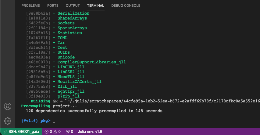
The plotting package is fairly large so this will take some time, but this only has to be done once.
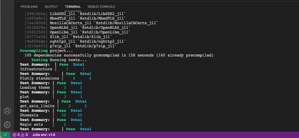
Once the installation is done, you can test whether the package works by running the build-in testing suite of that package (which is available for most julia packages):
(@v1.6) pkg> test Plots
This should look something like:
CTRL-C.
Once you are done with the package manager, go back to the REPL with the backspace button.
6. Create plots
Now that the plotting package is install, we are ready to create our first plot. First you load the Plots package
julia> using Plots
Next create a plot with
julia> plot(x,y)
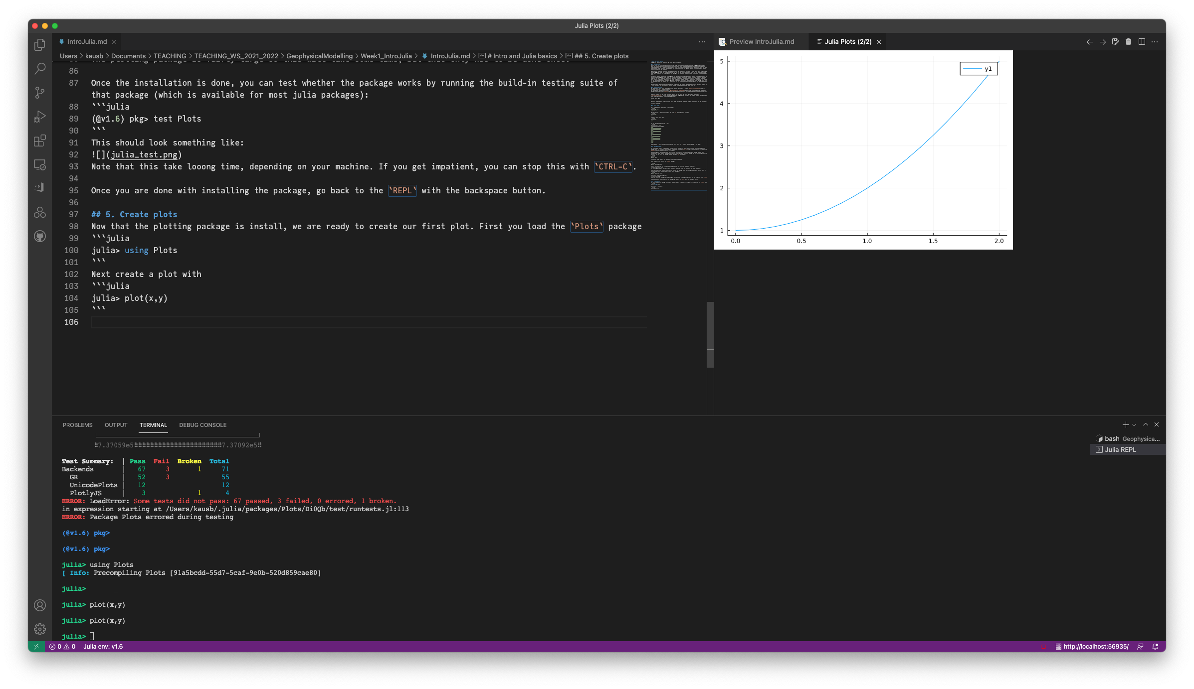
If you are using VSCode, it should show the plot in a seperate tab as in the figure above.
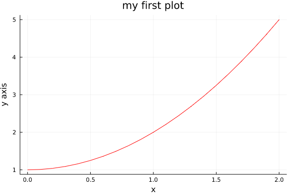
We can add labels etc. with:
julia> x=0:.1:2
julia> y=x.^2 .+ 1
julia>  plot(x,y, xlabel="x", ylabel="y axis", title="my first plot",label=:none, color=:red)
which gives:
There are lots of options within the plotting package. Have a look at the tutorial here. If you are used to work with MATLAB/Octave, here a quick summary of how plotting options are called in the Plots.jl package of julia:
| MATLAB/Octave | Julia |
|---|---|
| plot(x,y,‘r–’) | plot(x,y,linestyle=:dash, color=:red) |
| scatter(x,y) | scatter(x,y) |
| mesh(x,y,z) | wireframe(x,y,z) |
| surf(x,y,z) | plot(x,y,z,st=:surface) |
| pcolor(x,y,z) | heatmap(x,y,z) |
| contour(x,y,z,50) | contour(x,y,z,level=50) |
| contourf(x,y,z) | contour(x,y,z,level=50,fill=true) |
7. Functions
A function in julia can be defined in an extremely simple manner:
julia> f(x) = x.^2 .+ 10
f (generic function with 1 method)
You can now use this function with scalars, vectors or arrays:
julia> f(10)
110
julia> x=1:3
julia> f(x)
3-element Vector{Int64}:
  11
  14
  19
julia> y=[1 2; 3 4]
julia> f(y)
2×2 Matrix{Int64}:
 11  14
 19  26
Functions ofcourse don’t have to be one-liners, so you can also define it as:
julia> function f1(x)
         y = x.^2 .+ 11
         return y
       end
f1 (generic function with 1 method)
This creates a new array y and returns that.
So how fast is this function? Lets start with defining a large vector:
julia> x=1:1e6;
It turns out that julia has a handy macro, called @time, with which you can record the time that a function took.
julia> @time f1(x)
  0.091410 seconds (407.44 k allocations: 31.651 MiB, 9.82% gc time, 94.01% compilation time)
1000000-element Vector{Float64}:
 12.0
 15.0
 20.0
 27.0
 36.0
 47.0
 60.0
 75.0
 92.0
  ⋮
  9.9998600006e11
  9.99988000047e11
  9.99990000036e11
  9.99992000027e11
  9.9999400002e11
  9.99996000015e11
  9.99998000012e11
  1.000000000011e12
So this took 0.09 seconds on my machine. Yet, the first time any function in julia is executed, it is compiled and that’s why 94% of the time was the compilation time. If we run the same function again, it is much faster and creates 2 allocations:
julia> @time f1(x)
  0.006275 seconds (2 allocations: 7.629 MiB)
In general, it is a very good idea to put things in functions within julia, as it allows julia to precompile the routines.
Also note that you need to restart the REPL or your Julia session every time you redefine a function or a structure.
8. Scripts
In general, you want to put your code in a julia script so you don’t have to type it always in the REPL. Doing that is simple; you simple save it as a textfile that had has *.jl as an ending.
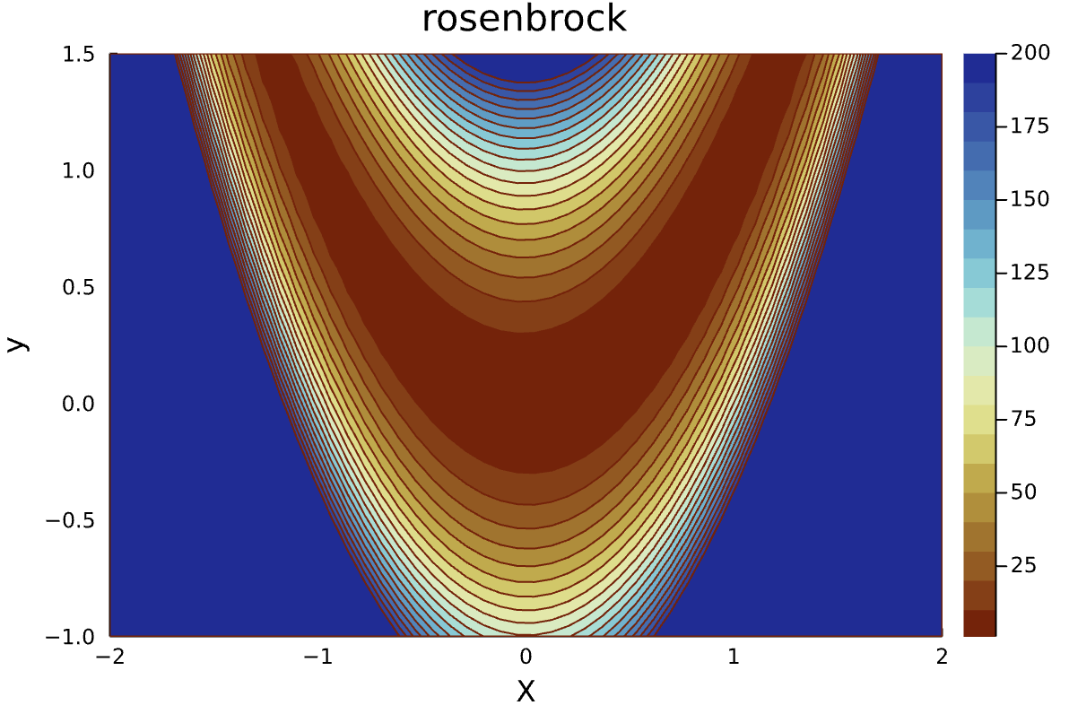
A simple example is the following test1.jl script:
using Plots

function rosenbrock(x,y; a=1,b=100)
   xt = x'     # transpose
   f  = (a .- xt).^2 .+ b.*(y .- xt.^2).^2
   return f
end

x = range(-2.0,2.0,length=50)
y = range(-1.0,1.5,length=50)
f = rosenbrock(x,y)

# Create a contourplot
contour(x,y,f, levels=0:10:200, fill=true,
       xlabel="X", ylabel="y", title="rosenbrock",
       color=:roma, clim=(1,200))
Note that the rosenbrock function has optional parameters (a,b). Calling it with only X,Y will invoke the default parameters, but you can specify the optional ones with f=rosenbrock(x,y, b=200,a=3).
You can run this script in the julia in the following way:
include("test1.jl")
Be aware that you need to be in the same directory as the script (see below on how you can change directories using the build-in shell in julia, by typing ; in the REPL).
The result looks like (have a look at how we customized the colormap, and added info for the axes).
9. Help
In general, you can get help for every function by typing ? which brings you to the help terminal. Next type the name of the function.
For example, lets find out how to compute the average of an array
julia>?mean
You can add help info to your own functions by adding comments before the function, using """
"""
    y = f2_withhelp(x)

Computes the square of `x` and adds 10

Example
=======

julia> x=1:10
julia> y = f2_withhelp(x)
10-element Vector{Int64}:
  11
  14
  19
  26
  35
  46
  59
  74
  91
 110
"""
function f2_withhelp(x)
    y = x.^2 .+ 10
    return y
end
9.1 Built-in terminal
Julia has a built-in terminal, which you can reach by typing ;. This comes in handy if you want to check in which directory you are, change directories, or look at the files there.
julia>;
shell> pwd
/Users/kausb
Note that this invokes the default terminal on your operating system, so under windows the commands are a but different than under linux.
Once you are done with the terminal, you get back to the REPL, by using the backspace.
9.2 Online help
The official julia manual is a good place to start. Many of the julia packages are hosted on github and have help pages as well. An example, which we will use in this class, is GeophysicalModelGenerator.jl.
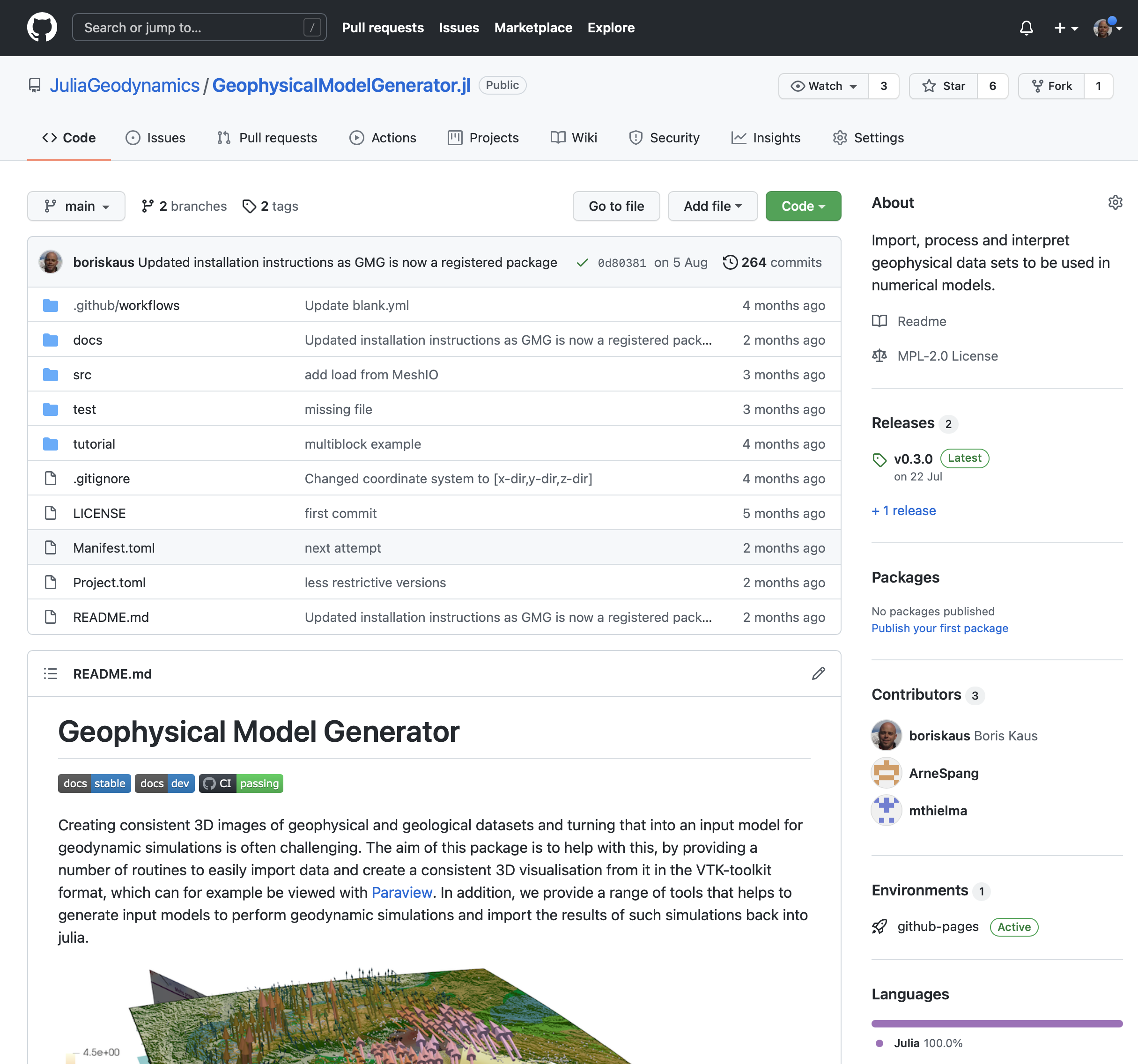
If you click on the blue buttons, you will be taken to the help pages.
10. Other useful packages
As you will work your way through the tutorials you will see that we often use external packages, for example to load ascii data files into julia. You will find detailed instructions in the respective tutorials.
The packages we will use in this tutorial are listed below.
- CSV: Read comma-separated data files into julia.
- Plots: Create all kinds of plots in julia (quite an extensive package, but very useful to have).
- JLD2: This allows saving julia objects (such as a tomographic model) to a binary file and load it again at a later stage.
- Geodesy: Convert UTM coordinates to latitude/longitude/altitude.
- NetCDF: Read NetCDF files.
- GMT: A julia interface to the Generic Mapping Tools (GMT), which is a highly popular package to create (geophysical) maps. Note that installing
GMT.jlis more complicated than installing the other packages listed above, as you first need to have a working version ofGMTon your machine (it is not yet installed automatically). Installation instructions for Windows/Linux are on their webpage. On a Mac, we made the best experiences by downloading the binaries from their webpage and not using a package manager to install GMT.
Install them through the package manager:
julia> using Pkg
julia> Pkg.add("CSV")
Marcel Thielmann
Principal Investigator/Group Leader
Working on localization processes in Earth materials, in particular deep earthquakes, flow of complex fluids in porous media and Earth’s lower mantle rheology.