Visualization

To show you how to visualize data, we will use one of the exmaples given in the GMG documentation. We will repeat it here for completeness. The example is the P-wave velocity model of the Alps as described in:

Zhao, L., Paul, A., Malusà, M.G., Xu, X., Zheng, T., Solarino, S., Guillot, S., Schwartz, S., Dumont, T., Salimbeni, S., Aubert, C., Pondrelli, S., Wang, Q., Zhu, R., 2016. Continuity of the Alpine slab unraveled by high-resolution P wave tomography. Journal of Geophysical Research: Solid Earth 121, 8720–8737. doi:10.1002/2016JB013310

The data is given in ASCII format with longitude/latitude/depth/velocity anomaly (percentage) format. You can find the processed data here.

1. Visualizing data with Paraview

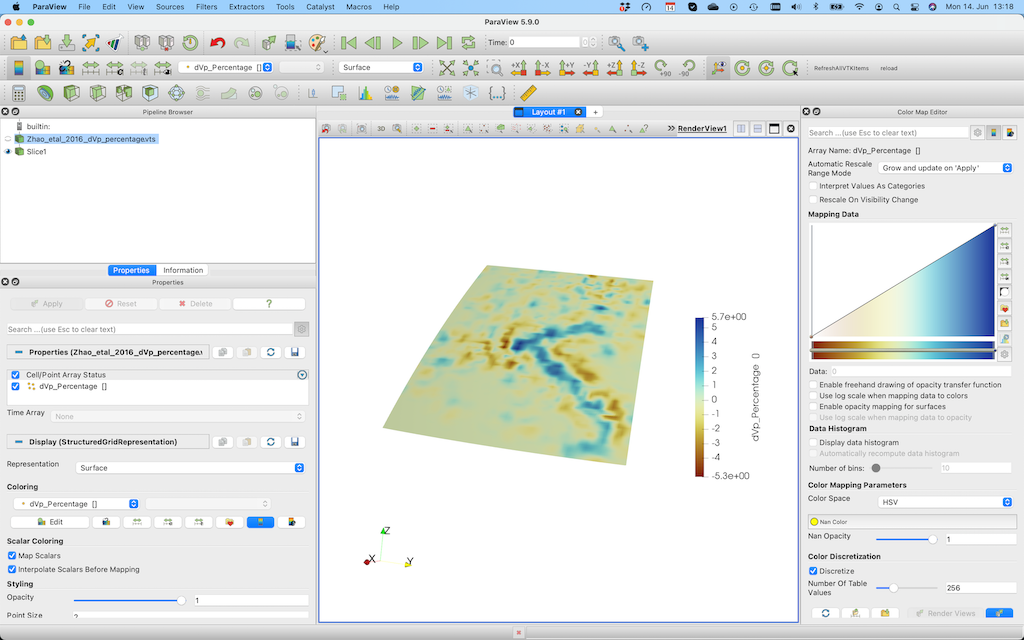
Importing data into Paraview is fairly straightforward, as one simply needs to open the desired vts file. In our case, open the file Zhao_etal_2016_dVp_percentage.vts. in Paraview. Press Apply (left menu) after doing that. Once you did that you can select dVp_Percentage and Surface (see red ellipses below)/.

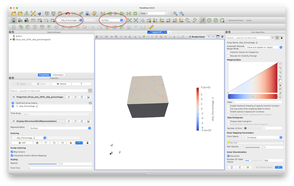
This visualisation employs the default colormap, which is not particularly good.

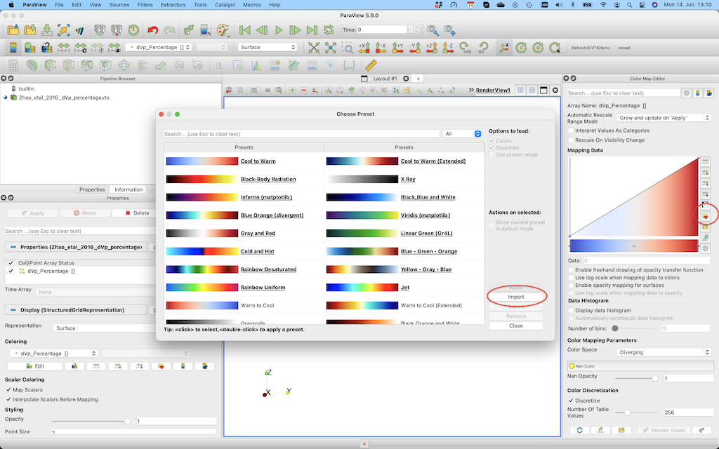
You can change that by importing the roma colormap (link). For this, open the colormap editor and click the one with the heart on the right hand side. Next, import roma and select it. Alternatively, use one of the already provided colormaps.

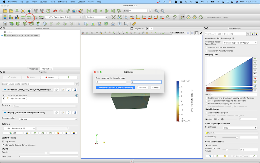
In order to change the color range select the button in the red ellipse and change the lower/upper bound.

If you want to create a horizontal cross-section @ 200 km depth, you need to select the Slice tool, select Sphere as a clip type, set the center to [0,0,0] and set the radius to 6171 (=radius earth - 200 km).

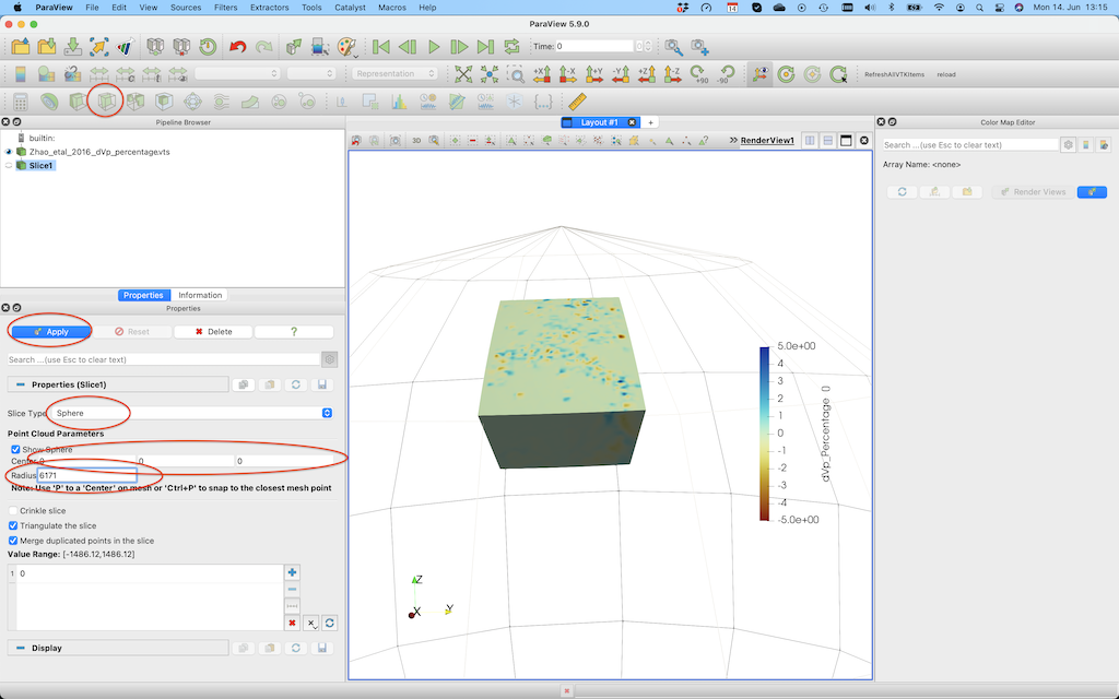
After pushing Apply, you’ll see this:

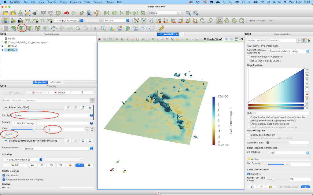
If you want to plot iso-surfaces (e.g. at -3%), you can use the Clip option again, but this time select scalar and don’t forget to unclick invert.

2. Visualizing cross sections

In principle, Paraview allows to create cross sections of given data. However, Paraview operates in Cartesian coordinates, which makes it difficult to create arbitrary cross-sections with given longitude and latitude. As we have already covered in this tutorial, there is a simple way to create cross sections using the CrossSection function. Here we will go through creating different cross-sections, exporting them and to visualize them in Paraview.

First, go to the directory where the data is located, start up julia and load the JLD2 and GeophyicalModelGenerator package. Then, load the data that we have already converted to GMG format:

julia> using  GeophysicalModelGenerator,JLD2
julia> load_object("Zhao_Pwave.jld2")

Below, we list the commands needed to create different cross-sections.

To make a cross-section at a given depth:

julia> Data_cross  =   CrossSection(Data_set, Depth_level=-100km)  
GeoData 
  size  : (121, 94, 1)
  lon   ϵ [ 0.0 : 18.0]
  lat   ϵ [ 38.0 : 51.95]
  depth ϵ [ -101.0 km : -101.0 km]
  fields: (:dVp_Percentage,)
julia> Write_Paraview(Data_cross, "Zhao_CrossSection_100km")
1-element Vector{String}:
 "Zhao_CrossSection_100km.vts"

Or at a specific longitude:

julia> Data_cross  =   CrossSection(Data_set, Lon_level=10)
GeoData 
  size  : (1, 94, 101)
  lon   ϵ [ 10.05 : 10.05]
  lat   ϵ [ 38.0 : 51.95]
  depth ϵ [ -1001.0 km : -1.0 km]
  fields: (:dVp_Percentage,) 
julia> Write_Paraview(Data_cross, "Zhao_CrossSection_Lon10")
1-element Vector{String}:
 "Zhao_CrossSection_Lon10.vts"

As you see, this cross-section is not taken at exactly 10 degrees longitude. That is because by default we don’t interpolate the data, but rather use the closest point in longitude in the original data set.

If you wish to interpolate the data, specify Interpolate=true:

julia> Data_cross  =   CrossSection(Data_set, Lon_level=10, Interpolate=true)
GeoData 
  size  : (1, 100, 100)
  lon   ϵ [ 10.0 : 10.0]
  lat   ϵ [ 38.0 : 51.95]
  depth ϵ [ -1001.0 km : -1.0 km]
  fields: (:dVp_Percentage,)
julia> Write_Paraview(Data_cross, "Zhao_CrossSection_Lon10_interpolated");

as you see, this causes the data to be interpolated on a (100,100) grid (which can be changed by adding a dims input parameter).

We can also create a diagonal cut through the model:

julia> Data_cross  =   CrossSection(Data_set, Start=(1.0,39), End=(18,50))
GeoData 
  size  : (100, 100, 1)
  lon   ϵ [ 1.0 : 18.0]
  lat   ϵ [ 39.0 : 50.0]
  depth ϵ [ -1001.0 km : -1.0 km]
  fields: (:dVp_Percentage,)
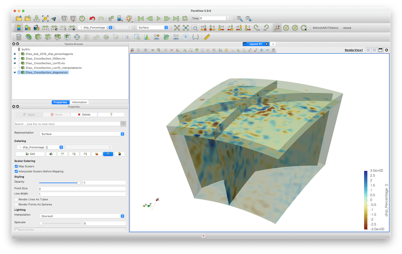
julia> Write_Paraview(Data_cross, "Zhao_CrossSection_diagonal")

Here an image that shows the resulting cross-sections:

3. Extract a (3D) subset of the data

Sometimes, the data set covers a large region (e.g., the whole Earth), and you are only interested in a subset of this data for your project. You can obviously cut your data to the correct size in Paraview. Yet, an even easier way is the routine ExtractSubvolume:

julia> Data_subset     =   ExtractSubvolume(Data_set,Lon_level=(5,12), Lat_level=(40,45))
GeoData 
  size  : (48, 35, 101)
  lon   ϵ [ 4.95 : 12.0]
  lat   ϵ [ 39.95 : 45.05]
  depth ϵ [ -1001.0 km : -1.0 km]
  fields: (:dVp_Percentage,)
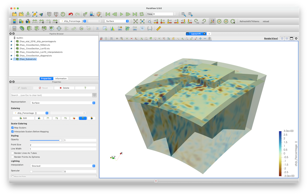
julia> Write_Paraview(Data_subset, "Zhao_Subset")

This gives the resulting image. You can obviously use that new, smaller, data set to create cross-sections etc.

By default, we extract the original data and do not interpolate it on a new grid. In some cases, you will want to interpolate the data on a different grid. Use the Interpolate=true option for that:

julia> Data_subset_interp     =   ExtractSubvolume(Data_set,Lon_level=(5,12), Lat_level=(40,45), Interpolate=true)
GeoData 
  size  : (50, 50, 50)
  lon   ϵ [ 5.0 : 12.0]
  lat   ϵ [ 40.0 : 45.0]
  depth ϵ [ -1001.0 km : -1.0 km]
  fields: (:dVp_Percentage,)
julia> Write_Paraview(Data_subset, "Zhao_Subset_interp")

If you need more colormaps or if you do not like the ones provided in Paraview, you can download additional colormaps for Paraview from Fabio Crameris website.

• Previous: Exporting data

• Back to the main page